Mostrando postagens com marcador Medium. Mostrar todas as postagens

sexta-feira, 1 de maio de 2020

New Features in Python 3.9 You Should Know About

Por Martin Heinz em 25/04/20 no site Medium


The release of Python 3.9 is still quite a while away (5.10.2020), but with the last alpha (3.9.0a5) release out and first beta in near future, it feels like it’s time to see what new features, improvements and fixes we can expect and look forward to. This article won’t be an exhaustive list of every change, but rather a list of the most interesting and noteworthy things to come with the next version for us — developers. So, let’s dive in!
Original Photo by David Clode on Unsplash

Installing Beta Version

wget https://www.python.org/ftp/python/3.9.0/Python-3.9.0a5.tgz
tar xzvf Python-3.9.0a5.tgz
cd Python-3.9.0a5
./configure --prefix=$HOME/python-3.9.0a5
make
make install
$HOME/python-3.9.0a5/bin/python3.9
After running this you should be greeted by IDLE and message like:
3.9.0a5 (default, Apr 16 2020, 18:57:58) 
[GCC 9.2.1 20191008] on linux
Type "help", "copyright", "credits" or "license" for more information.

New Dict Operators

# Dictionaries to be merged:
d1 = {"x": 1, "y": 4, "z": 10}
d2 = {"a": 7, "b": 9, "x": 5}

# Expected output after merging
{'x': 5, 'y': 4, 'z': 10, 'a': 7, 'b': 9}
# ^^^^^ Notice that "x" got overridden by value from second dictionary

# 1. Option
d = dict(d1, **d2)

# 2. Option
d = d1.copy()  # Copy the first dictionary
d.update(d2)   # Update it "in-place" with second one

# 3. Option
d = {**d1, **d2}
The first option above uses dict(iterable, **kwargs) function which initializes dictionaries - the first argument is a normal dictionary and the second one is a list of key/value pairs, in this case, it's just another dictionary unpacked using ** operator.
The second approach uses update function to update the first dictionary with pairs from the second one. As this one modifies dictionary in-place, we need to copy the first one into the final variable to avoid modifying the original.
Third — last — and in my opinion, the cleanest solution is to use dictionary unpacking and unpack both variables ( d1 and d2) into the resulting one d.
Even though the options above are completely valid, we now have a new (and better?) solution using | operator.
# Normal merging
d = d1 | d2
# d = {'x': 5, 'y': 4, 'z': 10, 'a': 7, 'b': 9}

# In-place merging
d1 |= d2
# d1 = {'x': 5, 'y': 4, 'z': 10, 'a': 7, 'b': 9}
The first example above does very much the same as operator unpacking shown previously ( d = {**d1, **d2}). The second example, on the other hand, can be used for in-place merging, where the original variable ( d1) is updated with values from the second operand ( d2).

Topological Ordering

Before the introduction of this feature, you would have to implement it yourself using e.g. Khan’s algorithm or depth-first search which aren’t exactly simple algorithms. So, now in case need to — for example — sort dependant jobs for scheduling, you just do the following:
from functools import TopologicalSorter
graph = {"A": {"D"}, "B": {"D"}, "C": {"E", "H"}, "D": {"F", "G", "H"}, "E": {"G"}}
ts = TopologicalSorter(graph)
list(ts.static_order())
# ['H', 'F', 'G', 'D', 'E', 'A', 'B', 'C']
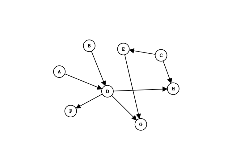
In the example above, we first create a graph using a dictionary, where keys are outgoing nodes and values are sets of their neighbours. After that, we create an instance of sorter using our graph and then call static_order function to produce the ordering. Bear in mind that this ordering may depend on the order of insertion because when 2 nodes are in the same level of the graph, they are going to be returned in the order they were inserted in.
Apart from static ordering, this class also supports parallel processing of nodes as they become ready for processing, which is useful when working with e.g. task queues — you can find examples of that in Python library docs here.

IPv6 Scoped Addresses

So, in case you need to deal with IPv6 addresses in Python, you can now do so like this:
from ipaddress import IPv6Address
addr = IPv6Address('ff02::fa51%1')
print(addr.scope_id)
# "1" - interface-local IP address
There is one thing you should be careful with when using IPv6 scopes though. Two addresses with different scopes are not equal when compared using basic Python operators.

New math Functions

import math

# Greatest common divisor
math.gcd(80, 64, 152)
# 8
Previously, the gcd function which calculates the Greatest Common Divisor could only be applied to 2 numbers, forcing programmers to do something like this math.gcd(80, math.gcd(64, 152)), when working with more numbers. Starting with Python 3.9, we can apply it to any number of values.
The first new addition to math module is math.lcm function:
# Least common multiple
math.lcm(4, 8, 5)
# 40
math.lcm calculates Least Common Multiple of its arguments. Same as with GCD, it allows a variable number of arguments.
The 2 remaining new functions are very much related. These are math.nextafter and math.ulp:
# Next float after 4 going towards 5
math.nextafter(4, 5)
4.000000000000001
# Next float after 9 going towards 0
math.nextafter(9, 0)
8.999999999999998

# Unit in the Last Place
math.ulp(1000000000000000)
0.125

math.ulp(3.14159265)
4.440892098500626e-16
The math.nextafter(x, y) function is pretty straightforward - it's next float after x going towards y while taking into consideration floating-point number precision.
The math.ulp on the other hand, might look a little weird... ULP stands for "Unit in the Last Place" and it's used as a measure of accuracy in numeric calculations. The shortest explanation is using an example:
Let’s imagine that we don’t have 64 bit computer. Instead, all we have is just 3 digits. With these 3 digits, we can represent a number like 3.14, but not 3.141. With 3.14, the nearest larger number that we can represent is 3.15, These 2 numbers differ by 1 ULP (Units at the last place), which is 0.1. So, what the math.ulp returns is equivalent of this example, but with actual precision of your computer. For proper example and explanation see nice writeup at https://matthew-brett.github.io/teaching/floating_error.html.

New String Functions

# Remove prefix
"someText".removeprefix("some")
# "Text"

# Remove suffix
"someText".removesuffix("Text")
# "some"
These 2 functions perform what you would otherwise achieve using string[len(prefix):] for prefix and string[:-len(suffix)] for suffix. These are very simple operations and therefore also very simple functions, but considering that you might perform these operations quite often, it’s nice to have built-in function that does it for you.

Bonus: HTTP Codes

import http

http.HTTPStatus.EARLY_HINTS
# <HTTPStatus.EARLY_HINTS: 103>

http.HTTPStatus.TOO_EARLY  
# <HTTPStatus.TOO_EARLY: 425>

http.HTTPStatus.IM_A_TEAPOT
# <HTTPStatus.IM_A_TEAPOT: 418>
Looking at these status codes, I can’t quite see why would you ever use them. That said, it’s great to finally have I’m a Teapot status code at our disposal. It’s a great quality of life improvement that I can now use http.HTTPStatus.IM_A_TEAPOT when returning this code from production server ( sarcasm, Please never do that...).

Conclusion

If you liked this article you should check you other of my Python articles below!

Resources

sexta-feira, 8 de dezembro de 2017

Data science with Python: Turn your conditional loops to Numpy vectors

Tirthajyoti Sarkar em 05/12/2017 no site Medium

Resultado de imagem para python

Python is fast emerging as the de-facto programming language of choice for data scientists. But unlike R or Julia, it is a general purpose language and does not have a functional syntax to start analyzing and transforming numerical data right out of the box. So, it needs specialized library.
Numpy, short for Numerical Python, is the fundamental package required for high performance scientific computing and data analysis in Python ecosystem. It is the foundation on which nearly all of the higher-level tools such as Pandasand scikit-learn are built. TensorFlow uses NumPy arrays as the fundamental building block on top of which they built their Tensor objects and graphflow for deep learning tasks (which makes heavy use of linear algebra operations on a long list/vector/matrix of numbers).
Many Numpy operations are implemented in C, avoiding the general cost of loops in Python, pointer indirection and per-element dynamic type checking. The speed boost depends on which operations you’re performing. For data science and modern machine learning tasks, this is an invaluable advantage.
My recent story about demonstrating the advantage of Numpy-based vectorization of simple data transformation task caught some fancy and was well received by readers. There was some interesting discussion on the utility of vectorization over code simplicity and such.
Now, mathematical transformation based on some predefined condition are fairly common in data science tasks. And it turns out one can easily vectorize simple blocks of conditional loops by first turning them into functions and then using numpy.vectorize method. In my previous article I showed an order of magnitude speed boost for numpy vectorization of simple mathematical transformation. For the present case, the speedup is less dramatic, as the internal conditional looping is still somewhat inefficient. However, there is at least 20–50% improvement in the execution time over other plain vanilla Python codes.
Here is the simple code to demonstrate it:
import numpy as np
from math import sin as sn
import matplotlib.pyplot as plt
import time
# Number of test points
N_point = 1000
# Define a custom function with some if-else loops
def myfunc(x,y):
if (x>0.5*y and y<0.3):
return (sn(x-y))
elif (x<0.5*y):
return 0
elif (x>0.2*y):
return (2*sn(x+2*y))
else:
return (sn(y+x))
# List of stored elements, generated from a Normal distribution
lst_x = np.random.randn(N_point)
lst_y = np.random.randn(N_point)
lst_result = []
# Optional plots of the data
plt.hist(lst_x,bins=20)
plt.show()
plt.hist(lst_y,bins=20)
plt.show()
# First, plain vanilla for-loop
t1=time.time()
for i in range(len(lst_x)):
x = lst_x[i]
y= lst_y[i]
if (x>0.5*y and y<0.3):
lst_result.append(sn(x-y))
elif (x<0.5*y):
lst_result.append(0)
elif (x>0.2*y):
lst_result.append(2*sn(x+2*y))
else:
lst_result.append(sn(y+x))
t2=time.time()
print("\nTime taken by the plain vanilla for-loop\n----------------------------------------------\n{} us".format(1000000*(t2-t1)))
# List comprehension
print("\nTime taken by list comprehension and zip\n"+'-'*40)
%timeit lst_result = [myfunc(x,y) for x,y in zip(lst_x,lst_y)]
# Map() function
print("\nTime taken by map function\n"+'-'*40)
%timeit list(map(myfunc,lst_x,lst_y))
# Numpy.vectorize method
print("\nTime taken by numpy.vectorize method\n"+'-'*40)
vectfunc = np.vectorize(myfunc,otypes=[np.float],cache=False)
%timeit list(vectfunc(lst_x,lst_y))
# Results
Time taken by the plain vanilla for-loop
----------------------------------------------
2000.0934600830078 us
Time taken by list comprehension and zip
----------------------------------------
1000 loops, best of 3: 810 µs per loop
Time taken by map function
----------------------------------------
1000 loops, best of 3: 726 µs per loop
Time taken by numpy.vectorize method
----------------------------------------
1000 loops, best of 3: 516 µs per loop
Notice that I have used %timeit Jupyter magic command everywhere I could write the evaluated expression in one line. That way I am effectively running at least 1000 loops of the same expression and averaging the execution time to avoid any random effect. Consequently, if you run this whole script in a Jupyter notebook, you may slightly different result for the first case i.e. plain vanilla for-loop execution, but the next three should give very consistent trend (based on your computer hardware).
We see the evidence that, for this data transformation task based on a series of conditional checks, the vectorization approach using numpy routinely gives some 20–50% speedup compared to general Python methods.
It may not seem a dramatic improvement, but every bit of time saving adds up in a data science pipeline and pays back in the long run! If a data science job requires this transformation to happen a million times, that may result in a difference between 2 days and 8 hours.
In short, wherever you have a long list of data and need to perform some mathematical transformation over them, strongly consider turning those python data structures (list or tuples or dictionaries) into numpy.ndarrayobjects and using inherent vectorization capabilities.
Numpy provides a C-API for even faster code execution but it takes away the simplicity of Python programming. This Scipy lecture note shows all the related options you have in this regard.
There is an entire open-source, online book on this topic by a French neuroscience researcher. Check it out here.

If you have any questions or ideas to share, please contact the author at tirthajyoti[AT]gmail.com. Also you can check author’s GitHub repositoriesfor other fun code snippets in Python, R, or MATLAB and machine learning resources. If you are, like me, passionate about machine learning/data science/semiconductors, please feel free to add me on LinkedIn.

segunda-feira, 9 de outubro de 2017

Machine Learning Fácil — Classificando gatos e cachorros em 5 passos.

Suzana Viana Mota
Em 21/09/2017 no site Medium

Resultado de imagem para learning machine

Machine Learning é uma técnica de Inteligência Artificial que permite que a máquina aprenda através de exemplos, exatamente como os seres humanos.
Pouca gente percebe, mas a Inteligência Artificial já faz parte do nosso dia a dia:
  • Os emails do seu Gmail já são classificados automaticamente como Spam ou Não Spam
  • O seu Facebook já é capaz de identificar o rosto de cada um dos seus amigos e marcá-los automaticamente nas fotos do rolê do final de semana
  • Quando você faz uma compra online e recebe sugestões de produtos que foram selecionados por uma máquina que se baseia nas suas escolhas anteriores.
Ok, então a gente já se aproveita das técnicas de Machine Learning, sem perceber, mas como essa coisa toda funciona na prática? É isso que a gente vai descobrir agora!
Você sabe me dizer o que é um gato? E o que é um cachorro?
Se você é um humano seria muito simples responder a esta questão, provavelmente desde criança você viu uma série de exemplos de miaus e au-aus e sem perceber você estava sendo treinado para realizar esta classificação.
A resolução de problemas de classificação utilizando aprendizado de máquina ou machine learning, seguem exatamente o mesmo princípio. Oferecemos vários exemplos para a máquina e indicamos o que é um gato e o que é um cachorro e a partir daí a máquina é capaz de identificar o padrão encontrado observando todos os exemplos anteriores.
Parece mágica, macumba ou ilusionismo, mas é pura ciência! Vamos lá entender a partir de um exemplo como isso funciona e em breve você será capaz de criar seus próprios algoritmos de classificação…

1. Definição do Problema:

A primeira coisa é ter claro o que queremos classificar, existem os casos clássicos que classificam emails como spam ou não spam, em imagens que reconhecem sorrisos ou não sorrisos e nos carros autônomos podemos classificar um terreno com aclive e sem aclive, entre tantos outros exemplos.
No nossso problema queremos identificar o que é um gato e por eliminação, se o bichinho não for um gato, vamos identificá-lo como cachorro. Você deve se perguntar o que diferencia um gato de um cachorro, algumas características extremamente similares, como o fato de todos ele terem 4 patas não vão nos ajudar nessa diferenciação, portanto devem ser evitadas.
Levantamos então, três características do nosso gato referência:
  • É fofinho?
  • Tem orelhinha pequena?
  • Faz miau?
Se a resposta para cada uma destas perguntas for SIM responderemos com 1 e se for NÃO responderemos com 0.
Classificando nossos gatos (bichinho 1, 2, 3)
Classificando nossos cachorros ( bichinho 4, 5, 6)

2. Definindo nosso dataset:

Agora vamos criar nosso dataset, os dados que vamos lidar, para isso devemos traduzir essa informação “humana” contida na nossa tabela, para uma linguagem que seja entendida pelas máquinas.
Vamos utilizar a linguagem Python e transformar cada bichinho em uma variável, em cada uma iremos inserir características já definidas na tabela.
O primeiro valor corresponde a pergunta: É fofinho? o segundo corresponde a tem orelhinha pequena? e o terceiro a faz miau? Para cada pergunta vamos preenchendo com os valores 1 para resposta SIM e 0 para a resposta NÃO. Então mãos a obra!
bichinho1 = [1, 1, 1]
bichinho2 = [1, 0, 1]
bichinho3 = [0, 1, 1]
bichinho4 = [1, 1, 0]
bichinho5 = [0, 1, 0]
bichinho6 = [0, 1, 0]
Foi bem tranquilo fazer esta tradução, certo? Agora só precisamos agrupar todos os nossos animaizinhos no nosso pequeno banco de dados. Para fazer isso vamos criar uma nova variável e colocar todos os nossos bichinhos lá dentro.
dados = [bichinho1, bichinho2, bichinho3, bichinho4, bichinho5, bichinho6]
O próximo passo é contar para a nossa máquina qual dos nossos bichinhos do dataset é gato e qual é cachorro. Observe que só definimos as características de cada um, agora continuamos seguindo a nossa tabela de referência e vamos informar para a máquina quem é quem.
Precisamos portanto colocar um label, um rótulo ou uma marcação em cada um dos itens do nosso dataset.
Como a máquina prefere lidar com números, vamos criar a seguinte convenção:
1 = Gato
-1 = Cachorro
Agora informamos a nossa convenção para a máquina:
marcacoes = [1, 1, 1, -1, -1, -1]
Falamos que os três primeiros bichinhos são gatos e os três últimos são cachorros, simples assim.

3. Criando modelos

Agora vamos começar a utilizar as técnicas de Machine Learning propriamente ditas.
Existem uma série de diferentes abordagens como SVM, Árvores de decisão, K-Nearest Neighbors, Naive Bayes entre tantas outras.
Neste exemplo vamos utilizar a Naive Bayes. A abordagem Naive Bayes é baseada no teorema de probabilidade de Bayes e tem como objetivo calcular a probabilidade que uma amostra desconhecida pertença a cada uma das classes possíveis, ou seja, predizer (ou adivinhar) a classe mais provável.
Devemos em primeiro lugar importar as funções necessárias através do comando:
from sklearn.naive_bayes import MultinomialNB
OBS: Caso você nao tenha instalado a biblioteca sklearn, instale através dos comandos:
pip install scikit-learn
ou utilizando o ambiente anaconda, com o comando:
conda install scikit-learn
Agora vamos criar o nosso modelo. Fazemos uma chamada da função do scikit-learn que já realiza a adequação dos nossos dados ao algoritmo de classificação Naive Bayes. E por fim, passamos os nossos dados e nossas marcações para o nosso modelo ser gerado. Ou seja, estamos passando todo o conhecimento para o algoritmo de classificação: estes são os nossos bichinhos (dataset) e eu os classifiquei de acordo com estas marcações.
modelo = MultinomialNB()
modelo.fit(dados,marcacoes)

4. Fazendo Predições

Agora queremos mostrar um novo bicho e identificar em qual categoria ele se enquadra: gato ou cachorro?
bicho_misterioso1 = [1, 1, 1]
bicho_misterioso2 = [1, 0, 0]
bicho_misterioso3 = [0, 0, 1]
Agrupamos todos os nossos bichos misteriosos numa única variável.
teste = [bicho_misterioso1, bicho_misterioso2, bicho_misterioso3]

5. Observando Resultados:

Agora vamos ver se o nosso classificador está trabalhando bem, para tanto passamos todos os nossos bichinhos misteriosos que estão na variável teste para a predição, para que a máquina tente “adivinhar” o resultado.
resultado = modelo.predict(teste)
E agora como vamos saber se a máquina chegou em uma classificação correta?
Vamos considerar que já sabemos as respostas para cada um dos bichos misteriosos, estamos querendo verificar se o nosso classificador vai funcionar bem.
O primeiro bicho misterioso é um gato. O segundo bicho misterioso é um cachorro. E o terceiro bicho misterioso é um gato também.
Agora vamos passar essa informação para a máquina criando o nosso marcacoes_teste.
marcacoes_teste = [1,-1, 1]
E para realmente verificar, vamos comparar o resultado com as nossas marcacoes_teste.
print(“Resultado: “)
print(resultado)
print (“Marcacoes: “)
print(marcacoes_teste)
Ao rodar o nosso Algoritmo vamos ter como resposta:
Resultado [ 1 1 1]
Marcações [1 -1 1]
Isso significa que a máquina chutou que os animais misteriosos são:
Resultado[ Gato, Gato, Gato]
e a resposta correta deveria ser
Marcacoes [Gato,Cachorro,Gato]
Nada mau para uma base de dados tão pequena! Quanto maior o dataset, maior a chance da máquina oferecer a resposta correta.
Portanto o nosso algoritmo tem a acurácia de 66,66%, ou seja, ele acertou 2 bichos misteriosos do nosso total de 3.
Você pode testar este mesmo algoritmo com diferentes abordagens de Machine Learning como SVM, Árvores de Decisão ou K-Nearest Neighbors, baixe o código e faça seus testes!
Caso este texto tenha sido útil, compartilhe a sua experiência aqui com a gente! Até a próxima :)
O código completo deste exemplo pode ser visto aqui: